MR Dictionary

One-sample MR or MR with individual-level data

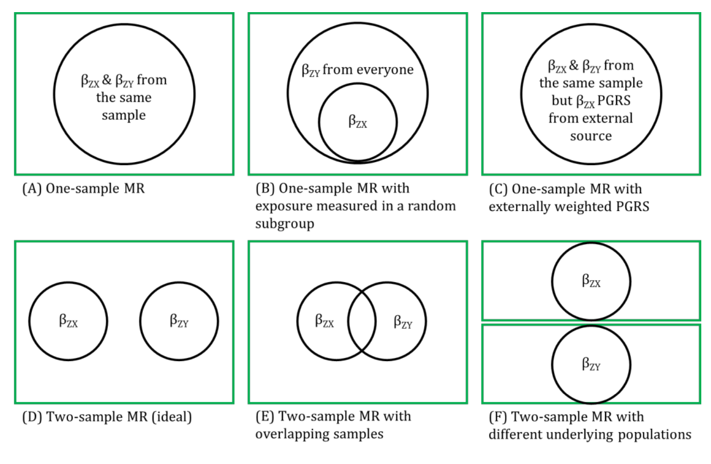
MR analyses in which the genetic instrumental variable (IV)-exposure association and genetic IV-outcome association are estimated from the same sample and individual-level data are used to derive the MR estimate.

Genetic IVs must fulfil the same MR assumptions. Genetic IVs (and weights for generating polygenic risk scores (PRSs), for example) associated with the exposure of interest are usually obtained from external data sources (e.g., a genome-wide association study (GWAS) of the exposure) and used within individual-level data (where the genetic IVs, exposure and outcome are measured) to generate a causal effect of the exposure on the outcome. In using individual-level data, there is more potential (than with two-sample MR) for assessing the associations between the genetic IV with observed confounders of the exposure-outcome association and exploring interactions, non-linear or subgroup effects. One-sample MR is more prone to data overfitting than two-sample MR. In one-sample MR, weak instrument bias will tend to bias the estimate towards the confounded multivariable regression estimate. Conversely, weak instrument bias in two-sample MR will tend to bias the estimate towards the null. Though, if there is overlap of participants in the two samples used for two-sample MR, the direction of any weak instrument bias in a two-sample setting will tend towards the confounded multivariable regression estimate (i.e., like in a one-sample setting with individual-level data) approximately proportional to the amount of overlap. The IV-exposure model can be miss-specified but the IV-outcome model must be correctly specified. NOTE: there are grey areas between one-sample MR and two-sample MR (e.g., in one-sample MR, when information from multiple data sources, such as betas from a GWAS that are used as weights in generating a PRS, is used to calculate an MR estimate with individual-level data, as shown in Figure 2.6). In fact, some MR studies use a mixture of analyses conducted in both individual- and summary-level data, sometimes using the same population sample. Therefore, the way in which these methods are described has evolved in the literature to focus on the data source being used in MR analyses rather than the number of samples - i.e., where "one-sample MR" is equivalent to "individual-level data MR" or "MR with individual-level data".

Relationship of one-sample and two-sample Mendelian randomization: populations and samples.  In all examples, the green box represents the same underlying population from which samples are drawn; the black circles represent the samples and the text in these summarises the source of association of genetic instrument with exposure (βZX) and association of genetic instrument with outcome (βZY). In one-sample MR (A) where βZX and βZY are estimated within the same population, there may be over-fitting of the data because the predicted (by genetic IV) values of X are then used to predict Y in the same sample. In this study type, weak instrument bias will be expected to bias towards the confounded result. In one-sample MR, it is not necessary to have exposures measured on all sample participants. For expensive exposures, these could be measured in a subsample (B). The properties and sources of bias will be broadly similar to those in (A), where exposures are measured in all participants, but the likelihood of weak instrument bias may be greater. When βZX is obtained in a one-sample MR study but with external weights (i.e., the
association magnitudes taken from a GWAS to which the sample being used for the MR did not contribute), as shown in (C), over-fitting of the data is minimised. Ideally, in two-sample MR, both samples are drawn from the same underlying population but there is no overlap of participants between the two samples, as shown in (D). In this situation, data will not be over-fitted and any weak instrument bias would be expected to bias towards the null. As GWAS get larger, and with more cohorts contributing to them, the potential for overlap between samples in summary data two-sample MR becomes increasingly likely, as shown in (E). The more overlap there is between the two samples, the more effects of over-fitting and weak instrument bias become similar to those seen in one-sample MR. In figure (F), the two samples are drawn from two different underlying populations. This might occur when using MR for testing developmental origins, when βZX is estimated in pregnant women and βZY is estimated in their offspring. In that situation, it is important to consider (and ideally test) whether the βZX association in pregnancy is the same as in non-pregnant females and males (i.e., as in the offspring sample). Similarly, when using aggregate data in two-sample MR and when the outcome of interest can only occur in one sex (e.g., cervical or prostate cancer), ideally one would want aggregate βZX estimates to be sex-specific. If that is not possible, then drawing on other external evidence to consider the extent to which βZX is likely to be similar in females and males is important.
Figure 2.6 - Relationship of one-sample and two-sample Mendelian randomization: populations and samples. In all examples, the green box represents the same underlying population from which samples are drawn; the black circles represent the samples and the text in these summarises the source of association of genetic instrument with exposure (βZX) and association of genetic instrument with outcome (βZY). In one-sample MR (A) where βZX and βZY are estimated within the same population, there may be over-fitting of the data because the predicted (by genetic IV) values of X are then used to predict Y in the same sample. In this study type, weak instrument bias will be expected to bias towards the confounded result. In one-sample MR, it is not necessary to have exposures measured on all sample participants. For expensive exposures, these could be measured in a subsample (B). The properties and sources of bias will be broadly similar to those in (A), where exposures are measured in all participants, but the likelihood of weak instrument bias may be greater. When βZX is obtained in a one-sample MR study but with external weights (i.e., the association magnitudes taken from a GWAS to which the sample being used for the MR did not contribute), as shown in (C), over-fitting of the data is minimised. Ideally, in two-sample MR, both samples are drawn from the same underlying population but there is no overlap of participants between the two samples, as shown in (D). In this situation, data will not be over-fitted and any weak instrument bias would be expected to bias towards the null. As GWAS get larger, and with more cohorts contributing to them, the potential for overlap between samples in summary data two-sample MR becomes increasingly likely, as shown in (E). The more overlap there is between the two samples, the more effects of over-fitting and weak instrument bias become similar to those seen in one-sample MR. In figure (F), the two samples are drawn from two different underlying populations. This might occur when using MR for testing developmental origins, when βZX is estimated in pregnant women and βZY is estimated in their offspring. In that situation, it is important to consider (and ideally test) whether the βZX association in pregnancy is the same as in non-pregnant females and males (i.e., as in the offspring sample). Similarly, when using aggregate data in two-sample MR and when the outcome of interest can only occur in one sex (e.g., cervical or prostate cancer), ideally one would want aggregate βZX estimates to be sex-specific. If that is not possible, then drawing on other external evidence to consider the extent to which βZX is likely to be similar in females and males is important.

References

Other terms in 'Definition of MR and study designs':