MR Dictionary

Directed acyclic graph (DAG)

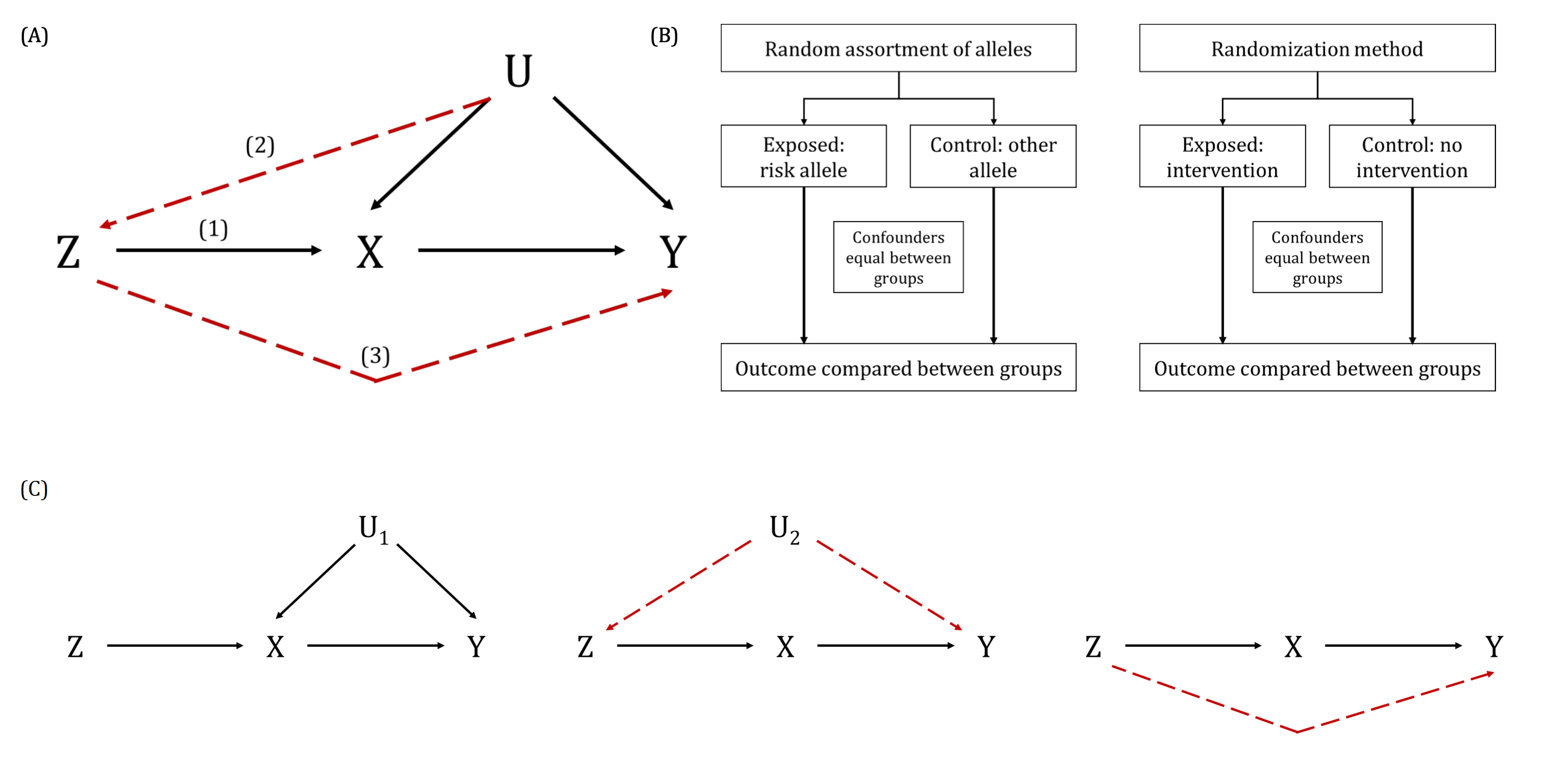
A DAG is a visual representation of potential causal relationships between variables. These relationships are demonstrated by nodes (representing variables) and arrows (a.k.a. edges or arches) between variables. The relationship between two variables in each DAG must be directed (i.e., there cannot be a bidirectional relationship). Relationships between all variables must be acyclic (i.e., a variable cannot have an impact on itself through any number of other variables).

DAGs are useful tools for explicitly demonstrating the underlying assumptions of a proposed analysis. Arrows are drawn between any two variables according to the following criteria: 1) An arrow from one variable to a second indicates that you assume that it is plausible that the first variable causes the second and 2) where there is no arrow between one variable and a second, this indicates that you assume that there is no causal relationship between the first and second variable. Thus, the three key assumptions of MR analyses are illustrated by an arrow from the instrumental variable (IV) to exposure; an absence of a variable that would have an arrow to the IV and to the outcome (i.e., no common cause of the IV and the outcome); and an absence of an arrow from the IV directly to the outcome.

Bidirectional Mendelian randomization. Adapted from Richmond et al. (A) In assessing whether physical activity (trait 1, represented by T1) causally influences body mass index (trait 2, represented by T2), genetic variants associated with physical activity (indicated by Z1) are used in an MR analysis. (B) In the reverse direction, genetic variants associated with body mass index (indicated by Z2) are used in an MR analysis to assess whether body mass index causally influences physical activity.
Figure 2.1 - Bidirectional Mendelian randomization. Adapted from Richmond et al. (A) In assessing whether physical activity (trait 1, represented by T1) causally influences body mass index (trait 2, represented by T2), genetic variants associated with physical activity (indicated by Z1) are used in an MR analysis. (B) In the reverse direction, genetic variants associated with body mass index (indicated by Z2) are used in an MR analysis to assess whether body mass index causally influences physical activity.
MR framework. (A) MR relies on the following three core assumptions: (1) the genetic variant(s) being used as an instrument (Z) is associated with the exposure (X) (often referred to as the relevance assumption); (2) there are no measured and unmeasured confounders of the instrument (Z) and the outcome (Y) (often referred to as the independence assumption); and (3) there is no independent pathway between the instrument (Z) and outcome (Y) other than through the exposure (X) (often referred to as the exclusion restriction or no horizontal pleiotropy assumption). (B) MR can be perceived as being analogous to a randomized controlled trial (RCT), whereby the random assortment of alleles at conception is equivalent to the randomization method with an RCT. This randomization process produces groups of individuals who differ with respect to the intervention (i.e., genetic variation in the case of MR) and between which confounders are equally distributed. Therefore, any differences observed in the outcome of interest between these randomly allocated groups should be due to the exposure with which the genetic variant(s) are associated. (C) Whilst, traditionally, the MR assumptions are usually depicted as in (A), this is a simplification of the three core assumptions and may be misleading. Consider the arrow linking the instrument (Z) and confounders of the exposure-outcome association (U) as depicted in (A). The random inheritance of alleles at conception provides genotypic groups at a population level between which confounders of the exposure-outcome association should be equally distributed. Coupled with the fact that confounders of the exposure-outcome association are unlikely to affect genetic variation, the arrow in this specific diagram realistically cannot go from U to Z (as depicted) but would, instead, pass from Z to U. However, this provides no distinction between the second and third MR assumptions, as described in (A). Instead, the second MR assumption refers to population-level confounders that could distort the relationship between the instrument and outcome, including intergenerational (e.g., dynastic ) effects, assortative mating or population structure or stratification. Therefore, to avoid this confusion, the three core MR assumptions are beginning to be depicted separately as in (C), where the first, second and third MR assumptions are depicted on the left, middle and right, respectively. Here, U1 represents confounders of the exposure-outcome association and U2 represents confounders of the instrument-outcome association, which are likely to be different from U1.
Figure 2.4 - MR framework. (A) MR relies on the following three core assumptions: (1) the genetic variant(s) being used as an instrument (Z) is associated with the exposure (X) (often referred to as the relevance assumption); (2) there are no measured and unmeasured confounders of the instrument (Z) and the outcome (Y) (often referred to as the independence assumption); and (3) there is no independent pathway between the instrument (Z) and outcome (Y) other than through the exposure (X) (often referred to as the exclusion restriction or no horizontal pleiotropy assumption). (B) MR can be perceived as being analogous to a randomized controlled trial (RCT), whereby the random assortment of alleles at conception is equivalent to the randomization method with an RCT. This randomization process produces groups of individuals who differ with respect to the intervention (i.e., genetic variation in the case of MR) and between which confounders are equally distributed. Therefore, any differences observed in the outcome of interest between these randomly allocated groups should be due to the exposure with which the genetic variant(s) are associated. (C) Whilst, traditionally, the MR assumptions are usually depicted as in (A), this is a simplification of the three core assumptions and may be misleading. Consider the arrow linking the instrument (Z) and confounders of the exposure-outcome association (U) as depicted in (A). The random inheritance of alleles at conception provides genotypic groups at a population level between which confounders of the exposure-outcome association should be equally distributed. Coupled with the fact that confounders of the exposure-outcome association are unlikely to affect genetic variation, the arrow in this specific diagram realistically cannot go from U to Z (as depicted) but would, instead, pass from Z to U. However, this provides no distinction between the second and third MR assumptions, as described in (A). Instead, the second MR assumption refers to population-level confounders that could distort the relationship between the instrument and outcome, including intergenerational (e.g., dynastic ) effects, assortative mating or population structure or stratification. Therefore, to avoid this confusion, the three core MR assumptions are beginning to be depicted separately as in (C), where the first, second and third MR assumptions are depicted on the left, middle and right, respectively. Here, U1 represents confounders of the exposure-outcome association and U2 represents confounders of the instrument-outcome association, which are likely to be different from U1.
Two-sample Mendelian randomization. Adapted from Hemani et al. (A) In two-sample MR, the associations of the instrument(s) with the exposure and outcome are derived from two independent (i.e., non-overlapping) samples. In this example, there are three SNPs acting as genetic IVs for the hypothetical exposure (i.e., SNP1, SNP2 and SNP3). (B) Manhattan plots showing the SNP-exposure estimates for each of the three SNPs are derived from a genome-wide association studies (GWAS) of the exposure variable. (C) The estimates of association between these three same SNPs and the outcome variable are then obtained from the outcome GWAS (results that are also depicted in a Manhattan plot). (D) Effects are harmonized to ensure that the ‘effect’ estimates in both the exposure and outcome GWASs correspond to the same allele (i.e., one that consistently either increases or decreases the exposure variable) for each SNP. (E) Once effects are harmonized, MR analyses can be performed. Visually, a scatter plot can be generated to represent the results, whereby the slope of the line is equivalent to the causal estimate. For example, the when using the inverse-variance weighted method, the intercept is held at zero.
Figure 2.5 - Two-sample Mendelian randomization. Adapted from Hemani et al. (A) In two-sample MR, the associations of the instrument(s) with the exposure and outcome are derived from two independent (i.e., non-overlapping) samples. In this example, there are three SNPs acting as genetic IVs for the hypothetical exposure (i.e., SNP1, SNP2 and SNP3). (B) Manhattan plots showing the SNP-exposure estimates for each of the three SNPs are derived from a genome-wide association studies (GWAS) of the exposure variable. (C) The estimates of association between these three same SNPs and the outcome variable are then obtained from the outcome GWAS (results that are also depicted in a Manhattan plot). (D) Effects are harmonized to ensure that the ‘effect’ estimates in both the exposure and outcome GWASs correspond to the same allele (i.e., one that consistently either increases or decreases the exposure variable) for each SNP. (E) Once effects are harmonized, MR analyses can be performed. Visually, a scatter plot can be generated to represent the results, whereby the slope of the line is equivalent to the causal estimate. For example, the when using the inverse-variance weighted method, the intercept is held at zero.
Two-step Mendelian randomization for exploring mediation. (A) In the first step of two-step MR, a genetic variant (Z1) is used as an instrument for the exposure of interest (X) to estimate the causal impact of the exposure on a hypothesized mediator (M) of the association between the exposure (X) and outcome (Y). (B) In the second step, an independent (of Z1) genetic variant (Z2) is used as an instrument for the mediator (M) to establish the causal impact of the mediator (M) on the outcome (Y). If there is evidence for a causal effect of X on M and M on Y (as well as X on Y), the estimates from these two steps can be combined to provide evidence for or against the mediating role of a variable on the exposure-outcome effect using e.g., multivariable MR.
Figure 2.7 - Two-step Mendelian randomization for exploring mediation. (A) In the first step of two-step MR, a genetic variant (Z1) is used as an instrument for the exposure of interest (X) to estimate the causal impact of the exposure on a hypothesized mediator (M) of the association between the exposure (X) and outcome (Y). (B) In the second step, an independent (of Z1) genetic variant (Z2) is used as an instrument for the mediator (M) to establish the causal impact of the mediator (M) on the outcome (Y). If there is evidence for a causal effect of X on M and M on Y (as well as X on Y), the estimates from these two steps can be combined to provide evidence for or against the mediating role of a variable on the exposure-outcome effect using e.g., multivariable MR.

References

Other terms in 'Related study designs and approaches ':