MR Dictionary

Horizontal Pleiotropy

A key way in which the exclusion restriction assumption may be violated. Also known as “genuine” or “true” pleiotropy. In MR, this is when a genetic variant influences the outcome (directly or indirectly, through other traits) independently of the hypothesised exposure. 

This can result in biased MR estimates because of violation of the exclusion restriction assumption. For example, if some or all of the genetic instrumental variables (IVs) that are robustly associated with an exposure of interest are also associated with other traits upstream of the outcome, independently of the exposure, then the MR estimate will be the combined (i.e., total) effect of all of these (independent) traits and not the (i.e., direct) effect of the exposure of interest alone. Methods such as MR-Egger, weighted median- and mode-based MR methods have been developed to explore and account for the impact of horizontal pleiotropy in MR studies. This can also be informative about the trait’s aetiology. There are further nuanced ways in which horizontal pleiotropy can lead to bias in MR analyses based on whether the pleiotropy is balanced or unbalanced, the latter of which is sometimes also known as directional pleiotropy. For example, if a subset of the genetic variants being used as instrumental variables (IVs) in an MR analysis have heterogenous causal effect estimates but these are equally balanced around the true causal effect (i.e., some have negative, some have positive effects), this balanced pleiotropy will likely not bias the resulting causal effect estimate. If, however, those genetic IVs have a consistent pleiotropic effect away from the true causal effect, this unbalanced pleiotropy will likely bias the derived causal effect estimate in a directional way.
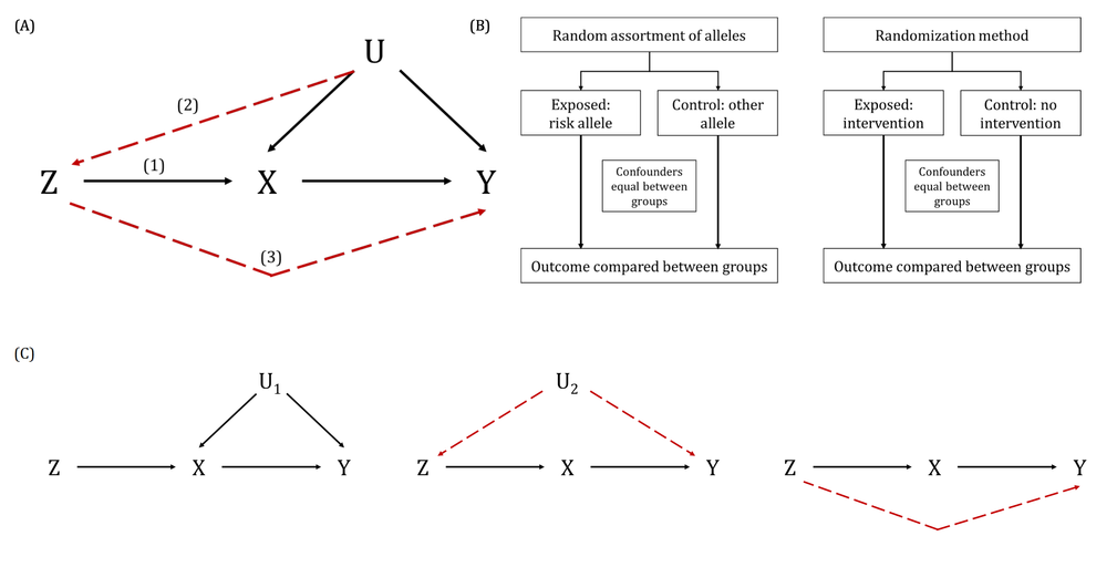
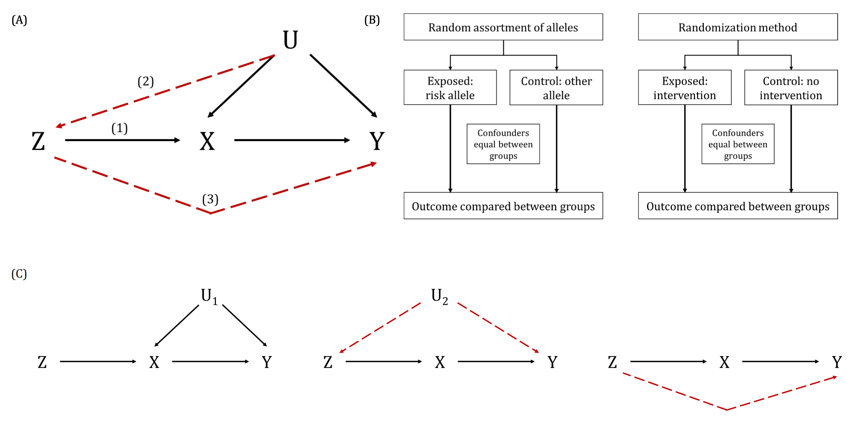
MR framework. (A) MR relies on the following three core assumptions: (1) the genetic variant(s) being used as an instrument (Z) is associated with the exposure (X) (often referred to as the relevance assumption); (2) there are no measured and unmeasured confounders of the instrument (Z) and the outcome (Y) (often referred to as the independence assumption); and (3) there is no independent pathway between the instrument (Z) and outcome (Y) other than through the exposure (X) (often referred to as the exclusion restriction or no horizontal pleiotropy assumption). (B) MR can be perceived as being analogous to a randomized controlled trial (RCT), whereby the random assortment of alleles at conception is equivalent to the randomization method with an RCT. This randomization process produces groups of individuals who differ with respect to the intervention (i.e., genetic variation in the case of MR) and between which confounders are equally distributed. Therefore, any differences observed in the outcome of interest between these randomly allocated groups should be due to the exposure with which the genetic variant(s) are associated. (C) Whilst, traditionally, the MR assumptions are usually depicted as in (A), this is a simplification of the three core assumptions and may be misleading. Consider the arrow linking the instrument (Z) and confounders of the exposure-outcome association (U) as depicted in (A). The random inheritance of alleles at conception provides genotypic groups at a population level between which confounders of the exposure-outcome association should be equally distributed. Coupled with the fact that confounders of the exposure-outcome association are unlikely to affect genetic variation, the arrow in this specific diagram realistically cannot go from U to Z (as depicted) but would, instead, pass from Z to U. However, this provides no distinction between the second and third MR assumptions, as described in (A). Instead, the second MR assumption refers to population-level confounders that could distort the relationship between the instrument and outcome, including intergenerational (e.g., dynastic ) effects, assortative mating or population structure or stratification. Therefore, to avoid this confusion, the three core MR assumptions are beginning to be depicted separately as in (C), where the first, second and third MR assumptions are depicted on the left, middle and right, respectively. Here, U1 represents confounders of the exposure-outcome association and U2 represents confounders of the instrument-outcome association, which are likely to be different from U1.
Figure 2.4 - MR framework. (A) MR relies on the following three core assumptions: (1) the genetic variant(s) being used as an instrument (Z) is associated with the exposure (X) (often referred to as the relevance assumption); (2) there are no measured and unmeasured confounders of the instrument (Z) and the outcome (Y) (often referred to as the independence assumption); and (3) there is no independent pathway between the instrument (Z) and outcome (Y) other than through the exposure (X) (often referred to as the exclusion restriction or no horizontal pleiotropy assumption). (B) MR can be perceived as being analogous to a randomized controlled trial (RCT), whereby the random assortment of alleles at conception is equivalent to the randomization method with an RCT. This randomization process produces groups of individuals who differ with respect to the intervention (i.e., genetic variation in the case of MR) and between which confounders are equally distributed. Therefore, any differences observed in the outcome of interest between these randomly allocated groups should be due to the exposure with which the genetic variant(s) are associated. (C) Whilst, traditionally, the MR assumptions are usually depicted as in (A), this is a simplification of the three core assumptions and may be misleading. Consider the arrow linking the instrument (Z) and confounders of the exposure-outcome association (U) as depicted in (A). The random inheritance of alleles at conception provides genotypic groups at a population level between which confounders of the exposure-outcome association should be equally distributed. Coupled with the fact that confounders of the exposure-outcome association are unlikely to affect genetic variation, the arrow in this specific diagram realistically cannot go from U to Z (as depicted) but would, instead, pass from Z to U. However, this provides no distinction between the second and third MR assumptions, as described in (A). Instead, the second MR assumption refers to population-level confounders that could distort the relationship between the instrument and outcome, including intergenerational (e.g., dynastic ) effects, assortative mating or population structure or stratification. Therefore, to avoid this confusion, the three core MR assumptions are beginning to be depicted separately as in (C), where the first, second and third MR assumptions are depicted on the left, middle and right, respectively. Here, U1 represents confounders of the exposure-outcome association and U2 represents confounders of the instrument-outcome association, which are likely to be different from U1.
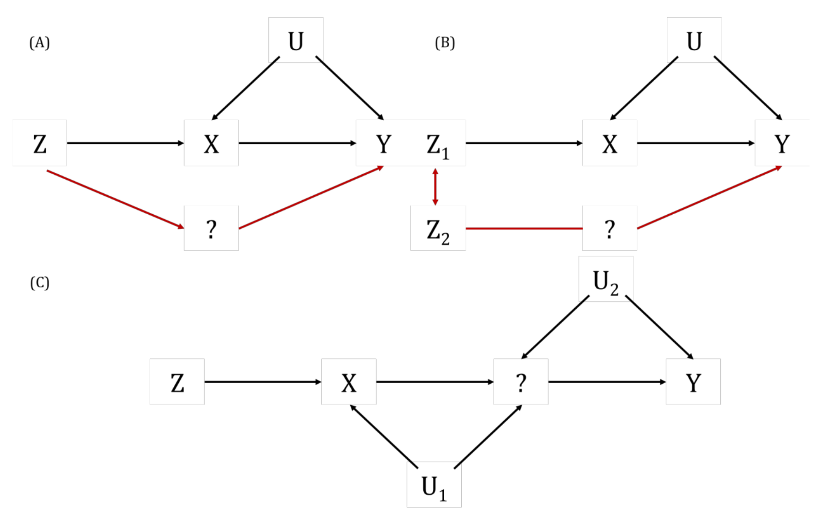
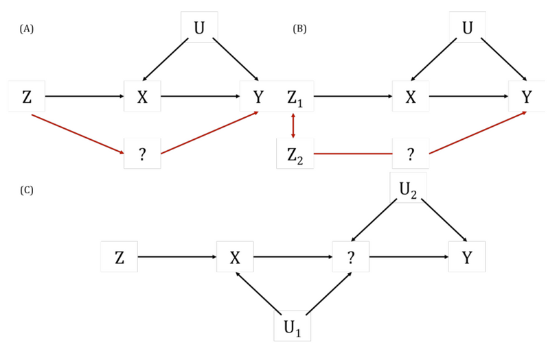
Vertical and Horizontal Pleiotropy. Adapted from Hemani et al.  and Holmes et al.  (A) Classic horizontal pleiotropy, whereby the instrument (Z) for the exposure of interest (X) is independently associated with the outcome (Y) either directly or indirectly through other trait(s) – denoted “?”. Here, this would violate the third assumption of MR and would bias results from an MR study. (B) Indirect horizontal pleiotropy, whereby another SNP (Z2) in linkage disequilibrium (LD) with the instrument (Z1) for the exposure of interest (X) is associated with the outcome (Y) and, due to this correlation between SNPs, the instrument is therefore not independent of the outcome of interest. This is another reason to use independent genetic variants as instruments in an MR analysis and to have some biological knowledge about the mechanisms by which the SNPs are associated with the exposure. (C) A depiction of vertical pleiotropy, whereby the genetic instrument (Z) for the exposure (X) is associated with other trait(s) – denoted “?” – however, this reflects the downstream effects of the exposure that is likely on the causal pathway linking the exposure to the outcome (Y). This is the very essence of MR and is not something that needs to be accounted for in analyses. Measured and unmeasured confounders in all diagrams as represented by “U”, “U1” and “U2”.
Figure 4.2 - Vertical and Horizontal Pleiotropy. Adapted from Hemani et al. and Holmes et al. (A) Classic horizontal pleiotropy, whereby the instrument (Z) for the exposure of interest (X) is independently associated with the outcome (Y) either directly or indirectly through other trait(s) – denoted “?”. Here, this would violate the third assumption of MR and would bias results from an MR study. (B) Indirect horizontal pleiotropy, whereby another SNP (Z2) in linkage disequilibrium (LD) with the instrument (Z1) for the exposure of interest (X) is associated with the outcome (Y) and, due to this correlation between SNPs, the instrument is therefore not independent of the outcome of interest. This is another reason to use independent genetic variants as instruments in an MR analysis and to have some biological knowledge about the mechanisms by which the SNPs are associated with the exposure. (C) A depiction of vertical pleiotropy, whereby the genetic instrument (Z) for the exposure (X) is associated with other trait(s) – denoted “?” – however, this reflects the downstream effects of the exposure that is likely on the causal pathway linking the exposure to the outcome (Y). This is the very essence of MR and is not something that needs to be accounted for in analyses. Measured and unmeasured confounders in all diagrams as represented by “U”, “U1” and “U2”.

References

Other terms in 'Sources of bias and limitations in MR':